How to Draw Line on Chart Excel

Note:The following procedure applies to Office 2013 and newer versions. Office 2010 steps?

Create a scatter chart

So, how did we create this scatter chart? The following procedure will help you create a scatter chart with similar results. For this chart, we used the example worksheet data. You can copy this data to your worksheet, or you can use your own data.

1. Copy the example worksheet data into a blank worksheet, or open the worksheet that contains the data you want to plot in a scatter chart.

   1 2 3 4 5 6 7 8 9 10 11

   A B Daily Rainfall Particulate 4.1 122 4.3 117 5.7 112 5.4 114 5.9 110 5.0 114 3.6 128 1.9 137 7.3 104

2. Select the data you want to plot in the scatter chart.

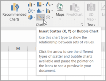
3. Click the Insert tab, and then click Insert Scatter (X, Y) or Bubble Chart.

   

4. Click Scatter.

   Tip:You can rest the mouse on any chart type to see its name.

5. Click the chart area of the chart to display the Design and Format tabs.

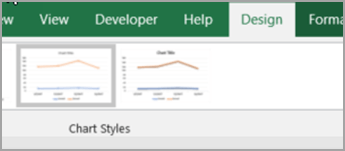
6. Click the Design tab, and then click the chart style you want to use.

   

7. Click the chart title and type the text you want.

8. To change the font size of the chart title, right-click the title, click Font, and then enter the size that you want in the Size box. Click OK.

9. Click the chart area of the chart.

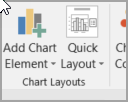
10. On the Design tab, click Add Chart Element > Axis Titles, and then do the following:

    

    1. To add a horizontal axis title, click Primary Horizontal.

    2. To add a vertical axis title, click Primary Vertical.

    3. Click each title, type the text that you want, and then press Enter.

    4. For more title formatting options, on the Format tab, in the Chart Elements box, select the title from the list, and then click Format Selection. A Format Title pane will appear. Click Size & Properties , and then you can choose Vertical alignment, Text direction, or Custom angle.

11. Click the plot area of the chart, or on the Format tab, in the Chart Elements box, select Plot Area from the list of chart elements.

    

12. On the Format tab, in the Shape Styles group, click the More button , and then click the effect that you want to use.

13. Click the chart area of the chart, or on the Format tab, in the Chart Elements box, select Chart Area from the list of chart elements.

14. On the Format tab, in the Shape Styles group, click the More button , and then click the effect that you want to use.

15. If you want to use theme colors that are different from the default theme that is applied to your workbook, do the following:

    1. On the Page Layout tab, in the Themes group, click Themes.

       

    2. Under Office, click the theme that you want to use.

Create a line chart

So, how did we create this line chart? The following procedure will help you create a line chart with similar results. For this chart, we used the example worksheet data. You can copy this data to your worksheet, or you can use your own data.

1. Copy the example worksheet data into a blank worksheet, or open the worksheet that contains the data that you want to plot into a line chart.

   1 2 3 4 5 6 7 8 9 10 11

   A B C Date Daily Rainfall Particulate 1/1/07 4.1 122 1/2/07 4.3 117 1/3/07 5.7 112 1/4/07 5.4 114 1/5/07 5.9 110 1/6/07 5.0 114 1/7/07 3.6 128 1/8/07 1.9 137 1/9/07 7.3 104

2. Select the data that you want to plot in the line chart.

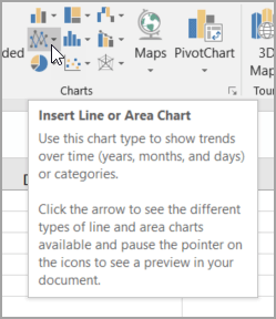
3. Click the Insert tab, and then click Insert Line or Area Chart.

   

4. Click Line with Markers.

5. Click the chart area of the chart to display the Design and Format tabs.

6. Click the Design tab, and then click the chart style you want to use.

   

7. Click the chart title and type the text you want.

8. To change the font size of the chart title, right-click the title, click Font, and then enter the size that you want in the Size box. Click OK.

9. Click the chart area of the chart.

10. On the chart, click the legend, or add it from a list of chart elements (on the Design tab, click Add Chart Element > Legend, and then select a location for the legend).

    

11. To plot one of the data series along a secondary vertical axis, click the data series, or select it from a list of chart elements (on the Format tab, in the Current Selection group, click Chart Elements).

    

12. On the Format tab, in the Current Selection group, click Format Selection. The Format Data Series task pane appears.

13. Under Series Options, select Secondary Axis, and then click Close.

14. On the Design tab, in the Chart Layouts group, click Add Chart Element, and then do the following:

    1. To add a primary vertical axis title, click Axis Title >Primary Vertical. and then on the Format Axis Title pane, click Size & Properties to configure the type of vertical axis title that you want.

    2. To add a secondary vertical axis title, click Axis Title > Secondary Vertical, and then on the Format Axis Title pane, click Size & Properties to configure the type of vertical axis title that you want.

    3. Click each title, type the text that you want, and then press Enter

15. Click the plot area of the chart, or select it from a list of chart elements (Format tab, Current Selection group, Chart Elements box).

16. On the Format tab, in the Shape Styles group, click the More button , and then click the effect that you want to use.

    

17. Click the chart area of the chart.

18. On the Format tab, in the Shape Styles group, click the More button , and then click the effect that you want to use.

19. If you want to use theme colors that are different from the default theme that is applied to your workbook, do the following:

    1. On the Page Layout tab, in the Themes group, click Themes.

       

    2. Under Office, click the theme that you want to use.

Create a scatter or line chart in Office 2010

So, how did we create this scatter chart? The following procedure will help you create a scatter chart with similar results. For this chart, we used the example worksheet data. You can copy this data to your worksheet, or you can use your own data.

1. Copy the example worksheet data into a blank worksheet, or open the worksheet that contains the data that you want to plot into a scatter chart.

   1 2 3 4 5 6 7 8 9 10 11

   A B Daily Rainfall Particulate 4.1 122 4.3 117 5.7 112 5.4 114 5.9 110 5.0 114 3.6 128 1.9 137 7.3 104

2. Select the data that you want to plot in the scatter chart.

3. On the Insert tab, in the Charts group, click Scatter.

   

4. Click Scatter with only Markers.

   Tip:You can rest the mouse on any chart type to see its name.

5. Click the chart area of the chart.

   This displays the Chart Tools, adding the Design, Layout, and Format tabs.

6. On the Design tab, in the Chart Styles group, click the chart style that you want to use.

   

   For our scatter chart, we used Style 26.

7. On the Layout tab, click Chart Title and then select a location for the title from the drop-down list.

   We chose Above Chart.

8. Click the chart title, and then type the text that you want.

   For our scatter chart, we typed Particulate Levels in Rainfall.

9. To reduce the size of the chart title, right-click the title, and then enter the size that you want in the Font Size box on the shortcut menu.

   For our scatter chart, we used 14.

10. Click the chart area of the chart.

11. On the Layout tab, in the Labels group, click Axis Titles, and then do the following:

    1. To add a horizontal axis title, click Primary Horizontal Axis Title, and then click Title Below Axis.

    2. To add a vertical axis title, click Primary Vertical Axis Title, and then click the type of vertical axis title that you want.

       For our scatter chart, we used Rotated Title.

       

    3. Click each title, type the text that you want, and then press Enter.

       For our scatter chart, we typed Daily Rainfall in the horizontal axis title, and Particulate level in the vertical axis title.

12. Click the plot area of the chart, or select Plot Area from a list of chart elements (Layout tab, Current Selection group, Chart Elements box).

13. On the Format tab, in the Shape Styles group, click the More button , and then click the effect that you want to use.

    For our scatter chart, we used the Subtle Effect - Accent 3.

    

14. Click the chart area of the chart.

15. On the Format tab, in the Shape Styles group, click the More button , and then click the effect that you want to use.

    For our scatter chart, we used the Subtle Effect - Accent 1.

16. If you want to use theme colors that are different from the default theme that is applied to your workbook, do the following:

    1. On the Page Layout tab, in the Themes group, click Themes.

       

    2. Under Built-in, click the theme that you want to use.

       For our line chart, we used the Office theme.

So, how did we create this line chart? The following procedure will help you create a line chart with similar results. For this chart, we used the example worksheet data. You can copy this data to your worksheet, or you can use your own data.

1. Copy the example worksheet data into a blank worksheet, or open the worksheet that contains the data that you want to plot into a line chart.

   1 2 3 4 5 6 7 8 9 10 11

   A B C Date Daily Rainfall Particulate 1/1/07 4.1 122 1/2/07 4.3 117 1/3/07 5.7 112 1/4/07 5.4 114 1/5/07 5.9 110 1/6/07 5.0 114 1/7/07 3.6 128 1/8/07 1.9 137 1/9/07 7.3 104

2. Select the data that you want to plot in the line chart.

3. On the Insert tab, in the Charts group, click Line.

   

4. Click Line with Markers.

5. Click the chart area of the chart.

   This displays the Chart Tools, adding the Design, Layout, and Format tabs.

6. On the Design tab, in the Chart Styles group, click the chart style that you want to use.

   

   For our line chart, we used Style 2.

7. On the Layout tab, in the Labels group, click Chart Title, and then click Above Chart.

   

8. Click the chart title, and then type the text that you want.

   For our line chart, we typed Particulate Levels in Rainfall.

9. To reduce the size of the chart title, right-click the title, and then enter the size that you want in the Size box on the shortcut menu.

   For our line chart, we used 14.

10. On the chart, click the legend, or select it from a list of chart elements (Layout tab, Current Selection group, Chart Elements box).

11. On the Layout tab, in the Labels group, click Legend, and then click the position that you want.

    For our line chart, we used Show Legend at Top.

12. To plot one of the data series along a secondary vertical axis, click the data series for Rainfall, or select it from a list of chart elements (Layout tab, Current Selection group, Chart Elements box).

13. On the Layout tab, in the Current Selection group, click Format Selection.

    

14. Under Series Options, select Secondary Axis, and then click Close.

15. On the Layout tab, in the Labels group, click Axis Titles, and then do the following:

    1. To add a primary vertical axis title, click Primary Vertical Axis Title, and then click the type of vertical axis title that you want.

       For our line chart, we used Rotated Title.

    2. To add a secondary vertical axis title, click Secondary Vertical Axis Title, and then click the type of vertical axis title that you want.

       For our line chart, we used Rotated Title.

    3. Click each title, type the text that you want, and then press ENTER.

       For our line chart, we typed Particulate level in the primary vertical axis title, and Daily Rainfall in the secondary vertical axis title.

16. Click the plot area of the chart, or select it from a list of chart elements (Layout tab, Current Selection group, Chart Elements box).

17. On the Format tab, in the Shape Styles group, click the More button , and then click the effect that you want to use.

    For our line chart, we used the Subtle Effect - Dark 1.

    

18. Click the chart area of the chart.

19. On the Format tab, in the Shape Styles group, click the More button , and then click the effect that you want to use.

    For our line chart, we used the Subtle Effect - Accent 3.

20. If you want to use theme colors that are different from the default theme that is applied to your workbook, do the following:

    1. On the Page Layout tab, in the Themes group, click Themes.

       

    2. Under Built-in, click the theme that you want to use.

       For our line chart, we used the Office theme.

How to Draw Line on Chart Excel

Source: https://support.microsoft.com/en-us/topic/present-your-data-in-a-scatter-chart-or-a-line-chart-4570a80f-599a-4d6b-a155-104a9018b86e

Share this post